Feedforward example
This page builds a feedforward neural network (NN) from a named
edgelist. You parse a directed acyclic graph (DAG)
with parse_layered(), write a module with one PackedLinear per
hop — everything arriving at one layer — train it
with ordinary PyTorch, and map attributions back to named nodes. If a
term is new, Concepts defines it.
Domain example: knowledge-primed neural networks
The key use case is the knowledge-primed neural network (KPNN), which gave the package its name. In a KPNN, prior knowledge encoded as a graph constrains the structure of a neural network: the model keeps only the connections that known relationships between named entities support. Each hidden node stands for one named entity, such as a transcription factor or a kinase. An attribution score on that node says how much the trained model relies on that entity's unit, rather than on an anonymous one; in a dense NN, only the input features have names.
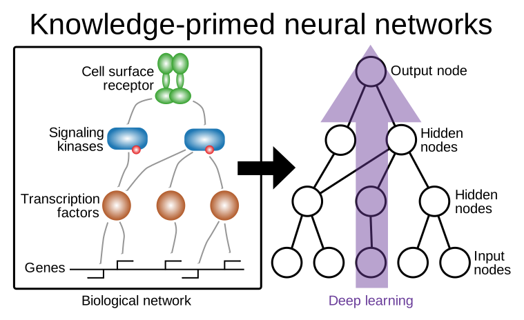
Figure 1. A pathway-based KPNN. The biological network on the left becomes the network on the right: genes are the input nodes, proteins such as kinases and transcription factors are named hidden nodes, the receptor is the output node, and every edge is a curated regulatory or signaling interaction.
KPNN examples include pathway-based models as in Fortelny and Bock, 2020 and ontology-based models such as in Elmarakeby et al., 2021. Biology is the example here, not the boundary: any architecture that can be written as named edges works the same way.
The kpnn2 workflow
An edgelist becomes a spec, the frozen structure a parser returns. You write a module around the spec, train it, and map attributions back onto the node names. The steps below follow that order:
- define a prior-knowledge edgelist
- parse it and write a
PackedLinearmodule - simulate data and align it to the model by name
- train the model with ordinary PyTorch, then save and reload it
- score the input features
- score the internal nodes
kpnn2 owns the structure and the names. Activations, the head, the
loss, the optimizer, the training loop, and the attribution method stay
yours. This notebook uses Captum, which kpnn2 does not import.
Installation
Install kpnn2 from PyPI with:
pip install kpnn2
The later interpretation cells also need Captum, which is not a
kpnn2 dependency:
pip install captum
Graphviz is used only to draw the toy graph in this notebook.
Imports
import numpy as np
import pandas as pd
import seaborn as sns
import torch
from graphviz import Digraph
from IPython.display import display
from matplotlib import pyplot as plt
from torch import nn

import kpnn2
import random

from matplotlib_inline.backend_inline import (
    set_matplotlib_formats,
)

random.seed(42)
np.random.seed(42)
torch.manual_seed(42)

set_matplotlib_formats(
    "svg",
    bbox_inches=None,
)
_FONT_SIZE = 14
_FIG_W = 7.0
_plot_rc = {
    "font.size": _FONT_SIZE,
    "axes.titlesize": _FONT_SIZE,
    "axes.labelsize": _FONT_SIZE,
    "xtick.labelsize": _FONT_SIZE,
    "ytick.labelsize": _FONT_SIZE,
    "legend.fontsize": _FONT_SIZE,
    "legend.title_fontsize": _FONT_SIZE,
    "lines.linewidth": 1.0,
    "font.family": "Liberation Sans",
    "text.color": "black",
    "axes.labelcolor": "black",
    "xtick.color": "black",
    "ytick.color": "black",
    "axes.edgecolor": "black",
    "axes.grid": False,
    "axes.facecolor": "none",
    "figure.facecolor": "none",
    "savefig.facecolor": "none",
    "savefig.edgecolor": "none",
    "svg.fonttype": "none",
}
plt.rcParams.update(_plot_rc)
sns.set_theme(
    style="ticks",
    rc=_plot_rc,
)


def _new_fig(height):
    return plt.figure(figsize=(_FIG_W, height))


def _style_ax(ax):
    ax.tick_params(labelsize=_FONT_SIZE)
    ax.title.set_fontsize(_FONT_SIZE)
    ax.xaxis.label.set_size(_FONT_SIZE)
    ax.yaxis.label.set_size(_FONT_SIZE)
    ax.set_facecolor("none")
    ax.grid(False)
Step 1: define a prior-knowledge edgelist
The architecture comes first, as a table of edges. A real prior comes from a curated database; here a handful of rows stands in for one.
kpnn2 expects an edgelist with two required columns, source and
target, one row per directed connection. Extra columns are ignored.
parse_layered() sorts nodes into layers by depth, which exists only
without feedback, so it requires the graph to be a DAG and raises on a
cycle. A graph with feedback loops goes through the other
parser, parse_adjacency(), shown in the Cyclic
graph example.
The example is a small feedforward biological graph with two clearly separated branches:
- a signal branch, connected to informative input features
- a noise branch, connected to uninformative input features
Keeping the branches apart is what makes the later interpretation steps easy to judge: after training, informative features and their connected hidden nodes should receive stronger attributions than the uninformative branch.
edgelist = pd.DataFrame(
    {
        "source": [
            "gene_signal_1",
            "gene_signal_2",
            "gene_signal_3",
            "gene_noise_1",
            "gene_noise_2",
            "gene_noise_3",
            "tf_signal",
            "tf_noise",
            "kinase_signal",
            "kinase_noise",
        ],
        "target": [
            "tf_signal",
            "tf_signal",
            "tf_signal",
            "tf_noise",
            "tf_noise",
            "tf_noise",
            "kinase_signal",
            "kinase_noise",
            "output_1",
            "output_1",
        ],
    }
)

edgelist
| source | target | |
|---|---|---|
| 0 | gene_signal_1 | tf_signal |
| 1 | gene_signal_2 | tf_signal |
| 2 | gene_signal_3 | tf_signal |
| 3 | gene_noise_1 | tf_noise |
| 4 | gene_noise_2 | tf_noise |
| 5 | gene_noise_3 | tf_noise |
| 6 | tf_signal | kinase_signal |
| 7 | tf_noise | kinase_noise |
| 8 | kinase_signal | output_1 |
| 9 | kinase_noise | output_1 |
# Visualize the graph

dot = Digraph()
dot.attr(rankdir="LR")

input_nodes = [
    "gene_signal_1",
    "gene_signal_2",
    "gene_signal_3",
    "gene_noise_1",
    "gene_noise_2",
    "gene_noise_3",
]
layer_1_nodes = ["tf_signal", "tf_noise"]
layer_2_nodes = ["kinase_signal", "kinase_noise"]
output_nodes = ["output_1"]

with dot.subgraph() as s:
    s.attr(rank="same")
    for node in input_nodes:
        s.node(node, node)

with dot.subgraph() as s:
    s.attr(rank="same")
    for node in layer_1_nodes:
        s.node(node, node)

with dot.subgraph() as s:
    s.attr(rank="same")
    for node in layer_2_nodes:
        s.node(node, node)

with dot.subgraph() as s:
    s.attr(rank="same")
    for node in output_nodes:
        s.node(node, node)

for _, row in edgelist.iterrows():
    dot.edge(row["source"], row["target"])

dot

Step 2: parse the edgelist and write a module
Parsing turns the table into the structure a module can be built
from. parse_layered(...) returns a LayeredSpec: named nodes by
layer, one packed hop per layer after the first, and metadata on
skip edges. It stops there and does not return an nn.Module.
Building the network is your job: one PackedLinear per hop, with your
own activations and task head around them. This spec has three hops and
no skip edges, so each hop reads only the layer below it. When an edge
jumps a layer, its hop reads more than one source layer and
gather_hop_inputs() concatenates them (see Skip
edges).
spec = kpnn2.parse_layered(edgelist)
spec.input_nodes, spec.hidden_nodes, spec.output_nodes
(('gene_noise_1',
  'gene_noise_2',
  'gene_noise_3',
  'gene_signal_1',
  'gene_signal_2',
  'gene_signal_3'),
 ('kinase_noise', 'kinase_signal', 'tf_noise', 'tf_signal'),
 ('output_1',))
Inspect the LayeredSpec
The three cells below read the parsed structure.
spec.layer_nodes[i] is the names at depth i, so the printed
tuples are the layers of the drawing above. spec.hops[i] is the
fixed packed connectivity entering layer i + 1, and it holds
every edge that arrives there, which is why the
(out_features, in_features) pairs are the shapes the three
PackedLinear layers will have. spec.skips is empty for this
graph, so every hop reads exactly the layer below it, and the
forward() below can pass x into lin0, that result into
lin1, and so on.
spec.layer_nodes
(('gene_noise_1',
  'gene_noise_2',
  'gene_noise_3',
  'gene_signal_1',
  'gene_signal_2',
  'gene_signal_3'),
 ('tf_noise', 'tf_signal'),
 ('kinase_noise', 'kinase_signal'),
 ('output_1',))
[(hop.out_features, hop.in_features) for hop in spec.hops]
[(2, 6), (2, 2), (1, 2)]
spec.skips
()
The model is a small nn.Module, and only its three PackedLinear
layers come from the spec, one per hop, named lin0, lin1, and
lin2. The graph ends in a single node, so a one-dimensional linear
head turns it into a single logit.
The module makes two choices about ReLU. ReLU is applied after
every hop except the last graph hop: output_1 is a scalar
bottleneck, and applying ReLU to it can suppress gradients if the
output is negative. ReLU can also zero a whole branch if that branch
starts with negative pre-activations. Both branches of this toy
graph should be able to learn, so each PackedLinear bias starts
at 1.0. Without that, the swap control later can fail even when
the labels sit on the noise-branch genes.
class KPNN(nn.Module):
    def __init__(self, spec: kpnn2.LayeredSpec):
        super().__init__()
        self.spec = spec
        self.lin0 = kpnn2.PackedLinear(
            spec.hops[0].source_index,
            spec.hops[0].target_index,
            spec.hops[0].out_features,
            spec.hops[0].in_features,
            identity=spec.fingerprint,
        )
        self.lin1 = kpnn2.PackedLinear(
            spec.hops[1].source_index,
            spec.hops[1].target_index,
            spec.hops[1].out_features,
            spec.hops[1].in_features,
            identity=spec.fingerprint,
        )
        self.lin2 = kpnn2.PackedLinear(
            spec.hops[2].source_index,
            spec.hops[2].target_index,
            spec.hops[2].out_features,
            spec.hops[2].in_features,
            identity=spec.fingerprint,
        )
        self.acts = nn.ModuleList([nn.ReLU() for _ in spec.hops])
        self.head = nn.Linear(1, 1)
        for layer in (self.lin0, self.lin1, self.lin2):
            if layer.bias is not None:
                nn.init.constant_(
                    layer.bias,
                    1.0,
                )

    def forward(self, x):
        h0 = self.acts[0](self.lin0(x))
        h1 = self.acts[1](self.lin1(h0))
        h2 = self.lin2(h1)
        return self.head(h2)


model = KPNN(spec)
model
KPNN(
  (lin0): PackedLinear(in_features=6, out_features=2, nnz=6, bias=True)
  (lin1): PackedLinear(in_features=2, out_features=2, nnz=2, bias=True)
  (lin2): PackedLinear(in_features=2, out_features=1, nnz=2, bias=True)
  (acts): ModuleList(
    (0-2): 3 x ReLU()
  )
  (head): Linear(in_features=1, out_features=1, bias=True)
)
Each hop is a PackedLinear, which keeps one trainable scalar per live
edge — an edge the graph actually has — instead
of a dense (out, in) matrix: layer.weight is one-dimensional, of
length nnz. MaskedLinear(hop.to_mask()) remains the dense hatch when
that rectangle fits. Each ReLU is an nn.ReLU module in self.acts,
not a function call inside forward(), so attribution methods that
treat nonlinearities specially can find it;
Mapping attributions says which.
Step 3: simulate data and align it to the model
PyTorch sees column positions, not names, so the tensor handed to
the model must follow the exact order stored in spec.input_nodes.
In practice, input data often comes from a DataFrame where features
are named but not necessarily ordered like the model input layer.
align_inputs() closes that gap: it returns a column index into
the caller's feature names. Gather with that index, then pass the
dense block to the model. This prevents silent feature-order
mismatches
between the data and the architecture.
The data is simulated here so that the interpretation steps have a
known answer. The gene_signal_* features carry class information,
while the gene_noise_* features are uninformative. The simulation
draws every feature from a normal distribution: the
gene_signal_* features use a different mean in each class, so
there is a real class difference the model can exploit, while the
gene_noise_* features use the same mean in both classes, so any
apparent difference between the classes is only random sampling
variation.
# Simulate the training and test data
rng = np.random.default_rng(42)

informative_features = [
    "gene_signal_1",
    "gene_signal_2",
    "gene_signal_3",
]

noise_features = [
    "gene_noise_1",
    "gene_noise_2",
    "gene_noise_3",
]

all_features = informative_features + noise_features

n_train_per_class = 100
n_test_per_class = 50


def simulate_binary_classification_data(n_per_class, rng):
    x0_signal = rng.normal(
        loc=0.0,
        scale=1.0,
        size=(n_per_class, len(informative_features)),
    )
    x1_signal = rng.normal(
        loc=2.0,
        scale=1.0,
        size=(n_per_class, len(informative_features)),
    )
    x0_noise = rng.normal(
        loc=0.0,
        scale=1.0,
        size=(n_per_class, len(noise_features)),
    )
    x1_noise = rng.normal(
        loc=0.0,
        scale=1.0,
        size=(n_per_class, len(noise_features)),
    )
    x0 = np.concatenate([x0_signal, x0_noise], axis=1)
    x1 = np.concatenate([x1_signal, x1_noise], axis=1)
    x = np.concatenate([x0, x1], axis=0)
    y = np.concatenate(
        [
            np.zeros(n_per_class, dtype=int),
            np.ones(n_per_class, dtype=int),
        ]
    )
    permutation = rng.permutation(len(y))
    x = x[permutation]
    y = y[permutation]
    x_df = pd.DataFrame(x, columns=all_features)
    y_series = pd.Series(y, name="label")
    return x_df, y_series


x_train_df, y_train = simulate_binary_classification_data(
    n_per_class=n_train_per_class,
    rng=rng,
)
x_test_df, y_test = simulate_binary_classification_data(
    n_per_class=n_test_per_class,
    rng=rng,
)

display(x_train_df.head())
display(y_train.head())
display(x_test_df.head())
display(y_test.head())
| gene_signal_1 | gene_signal_2 | gene_signal_3 | gene_noise_1 | gene_noise_2 | gene_noise_3 | |
|---|---|---|---|---|---|---|
| 0 | -0.695943 | -0.223859 | 0.242497 | -1.139429 | -0.481241 | 1.437777 |
| 1 | 3.068472 | 2.232878 | 2.234401 | -0.712102 | 1.370541 | -0.484030 |
| 2 | -0.471525 | 0.263717 | 0.052467 | 0.288917 | 1.244947 | -0.431339 |
| 3 | 0.941464 | 1.874991 | 3.481456 | -0.109727 | -0.035611 | -1.364742 |
| 4 | -0.926576 | -0.389810 | -1.376686 | -1.119536 | 0.447814 | 0.058274 |
0    0
1    1
2    0
3    1
4    0
Name: label, dtype: int64
| gene_signal_1 | gene_signal_2 | gene_signal_3 | gene_noise_1 | gene_noise_2 | gene_noise_3 | |
|---|---|---|---|---|---|---|
| 0 | -0.306566 | -0.593220 | -0.325545 | -0.491747 | 0.892856 | -0.774510 |
| 1 | 1.687645 | 3.358121 | 2.508079 | 0.619105 | -1.160912 | 0.032370 |
| 2 | -0.379687 | 0.376948 | -1.126988 | 1.191390 | -0.696212 | 0.223967 |
| 3 | 0.466178 | -0.376212 | -0.507105 | -1.567177 | 0.388474 | -1.759816 |
| 4 | 1.239810 | 2.577403 | 2.046557 | -1.466186 | -1.093737 | 1.026906 |
0    0
1    1
2    0
3    0
4    1
Name: label, dtype: int64
# Visualize the simulated training data

plot_df = x_train_df.copy()
plot_df["label"] = y_train.values
plot_df["class"] = plot_df["label"].map({0: "class 0", 1: "class 1"})

long_df = plot_df.melt(
    id_vars=["label", "class"],
    value_vars=spec.input_nodes,
    var_name="feature",
    value_name="value",
)

feature_type_map = {
    "gene_signal_1": "informative",
    "gene_signal_2": "informative",
    "gene_signal_3": "informative",
    "gene_noise_1": "uninformative",
    "gene_noise_2": "uninformative",
    "gene_noise_3": "uninformative",
}
long_df["feature_type"] = long_df["feature"].map(feature_type_map)

n_cols = 3
g = sns.catplot(
    data=long_df,
    x="class",
    y="value",
    col="feature",
    col_wrap=n_cols,
    hue="class",
    kind="box",
    width=0.35,
    sharey=False,
    height=3.3,
    aspect=1.0,
    legend=False,
)
g.fig.set_size_inches(_FIG_W, g.fig.get_figheight())
g.fig.suptitle(
    "Simulated training data: informative vs. uninformative features",
    fontsize=_FONT_SIZE,
    y=0.98,
)
g.fig.subplots_adjust(
    top=0.88,
    bottom=0.08,
    left=0.08,
    right=0.98,
    hspace=0.85,
    wspace=0.3,
)
for ax, feature in zip(g.axes.flat, spec.input_nodes):
    feature_type = feature_type_map[feature]
    ax.set_title(f"{feature}\n({feature_type})")
    ax.set_xlabel("")
    ax.set_ylabel("value")
    _style_ax(ax)
g.fig.patch.set_facecolor("none")
plt.show()

# Train and test share column order, so one col is valid.
col = kpnn2.align_inputs(x_train_df.columns, spec)
x_train = torch.as_tensor(
    x_train_df.to_numpy()[:, col],
    dtype=torch.float32,
)
x_test = torch.as_tensor(
    x_test_df.to_numpy()[:, col],
    dtype=torch.float32,
)
x_train.shape, x_test.shape
(torch.Size([200, 6]), torch.Size([100, 6]))
To check that alignment goes by name, the next cell reverses the DataFrame columns and aligns the reversed table again. The result is identical to the original aligned tensor.
# Alignment is name-based, not position-based.
# Even if the DataFrame columns are shuffled, the aligned tensor
# is unchanged.

shuffled_columns = list(reversed(spec.input_nodes))
x_train_df_shuffled = x_train_df[shuffled_columns]
x_train_from_shuffled = torch.as_tensor(
    x_train_df_shuffled.to_numpy()[
        :,
        kpnn2.align_inputs(
            x_train_df_shuffled.columns,
            spec,
        ),
    ],
    dtype=torch.float32,
)
torch.allclose(x_train, x_train_from_shuffled)
True
Keep this model with this spec. PyTorch never sees feature
names: column i of the input tensor is whatever name
spec.input_nodes[i] holds. To build each train, validation, or
test tensor, apply align_inputs() to that table's feature names.
Do not pass df.values, or any array you ordered by hand, to the
model. If the width is right, training still runs and the features
are silently wired to the wrong nodes. Extra columns and a shuffled
column order are fine; a renamed required column raises. A shared
col across splits is valid only when those tables have the same
column order; otherwise compute col from each table's names.
Step 4: train the model in PyTorch
Training is where kpnn2 steps back. The KPNN module is still a
normal PyTorch module, so it trains with ordinary PyTorch
components such as loss functions, optimizers, and training loops,
none of which the package provides.
Below is a minimal training loop that shows how the packed structural core and the added head fit directly into a standard PyTorch workflow.
# Train the model with the simulated data

y_train_tensor = torch.tensor(
    y_train.values.reshape(-1, 1),
    dtype=torch.float32,
)

optimizer = torch.optim.Adam(
    model.parameters(),
    lr=1e-2,
)
loss_fn = nn.BCEWithLogitsLoss()

n_epochs = 150
loss_history = []
model.train()

for epoch in range(n_epochs):
    optimizer.zero_grad()
    logits = model(x_train)
    loss = loss_fn(logits, y_train_tensor)
    loss.backward()
    optimizer.step()
    loss_history.append(loss.item())

print("Loss before first update:", round(loss_history[0], 4))
print("Loss after final update: ", round(loss_history[-1], 4))

_new_fig(2.8)
plt.plot(
    range(1, n_epochs + 1),
    loss_history,
    linewidth=1,
)
plt.xlabel("Epoch")
plt.ylabel("Binary cross-entropy loss")
plt.title("Training loss")
plt.tight_layout()
plt.show()
Loss before first update: 0.7193
Loss after final update:  0.1264

Save and reload the trained model
To reuse the trained model, save the spec together with the
weights. A state_dict carries numbers and no node names, so a
checkpoint is spec.to_dict() plus state_dict. The cell below
saves both, rebuilds the spec with LayeredSpec.from_dict(),
builds a fresh KPNN from it, and loads the weights. The
interpretation steps below run on that reloaded model. Each layer
was built with identity=spec.fingerprint, so loading a
checkpoint from a different prior raises instead of succeeding.
import tempfile

path = tempfile.NamedTemporaryFile(
    suffix=".pt",
    delete=False,
).name
payload = {
    "spec": spec.to_dict(),
    "state_dict": model.state_dict(),
}
torch.save(
    payload,
    path,
)
blob = torch.load(
    path,
    weights_only=False,
)
spec = kpnn2.LayeredSpec.from_dict(blob["spec"])
model = KPNN(spec)
model.load_state_dict(blob["state_dict"])
<All keys matched successfully>
Step 5: feature-level interpretation
The first question to ask a trained KPNN is which input features
drove its predictions. Any attribution method applies, because the
model is plain PyTorch; this example uses Captum
IntegratedGradients on the trained module. kpnn2 does not wrap
Captum.
The result is a tensor of shape (n_test, n_input_nodes) whose
columns follow spec.input_nodes, the same order
align_inputs indexes into, so the scores line up with the feature names. Those
values are signed Captum scores. The mean_abs_attribution column
below is computed with .abs() for ranking.
Simulation gives this step a ground truth: the gene_signal_*
features were generated with different class means, whereas the
gene_noise_* features were not. The recovered attributions need
not match those class mean differences exactly, but the informative
features should generally receive larger magnitudes than the
uninformative ones. That is the sanity check the table and plot
below are for.
from captum.attr import IntegratedGradients

model.eval()
ig = IntegratedGradients(model)
feature_tensor = ig.attribute(
    x_test,
    target=0,
)
feature_attr = pd.DataFrame(
    feature_tensor.detach().cpu().numpy(),
    columns=spec.input_nodes,
)
feature_attr.head()
| gene_noise_1 | gene_noise_2 | gene_noise_3 | gene_signal_1 | gene_signal_2 | gene_signal_3 | |
|---|---|---|---|---|---|---|
| 0 | 0.196101 | 0.668750 | 0.202322 | -0.497082 | -1.020986 | -1.048680 |
| 1 | -0.123444 | -0.434762 | -0.004228 | 1.538033 | 3.248478 | 4.541016 |
| 2 | -0.252323 | -0.276943 | -0.031072 | -0.615644 | 0.648761 | -3.630373 |
| 3 | 0.624964 | 0.290968 | 0.459710 | 0.755886 | -0.647495 | -1.633541 |
| 4 | 0.584690 | -0.819210 | -0.268255 | 1.429201 | 3.153695 | 4.686942 |
# Summarize feature attributions and compare them to the simulated
# signal

class_mean_diff = (
    x_test_df.loc[y_test == 1].mean() - x_test_df.loc[y_test == 0].mean()
)

feature_summary = pd.DataFrame(
    {
        "feature": spec.input_nodes,
        "abs_class_mean_difference": (
            class_mean_diff.abs().reindex(spec.input_nodes).values
        ),
        "mean_abs_attribution": (
            feature_attr.abs().mean(axis=0).reindex(spec.input_nodes).values
        ),
        "mean_signed_attribution": (
            feature_attr.mean(axis=0).reindex(spec.input_nodes).values
        ),
    }
)
feature_summary["feature_type"] = feature_summary["feature"].map(
    feature_type_map
)
feature_summary
| feature | abs_class_mean_difference | mean_abs_attribution | mean_signed_attribution | feature_type | |
|---|---|---|---|---|---|
| 0 | gene_noise_1 | 0.223047 | 0.307921 | 0.125116 | uninformative |
| 1 | gene_noise_2 | 0.251055 | 0.471399 | 0.035299 | uninformative |
| 2 | gene_noise_3 | 0.089079 | 0.187093 | 0.033711 | uninformative |
| 3 | gene_signal_1 | 2.086208 | 1.851277 | 1.198257 | informative |
| 4 | gene_signal_2 | 1.477629 | 1.977181 | 1.316618 | informative |
| 5 | gene_signal_3 | 1.617368 | 3.452763 | 2.320762 | informative |
# Plot recovered attributions against the true simulated signal

plot_df = feature_summary.melt(
    id_vars=["feature", "feature_type"],
    value_vars=[
        "abs_class_mean_difference",
        "mean_abs_attribution",
    ],
    var_name="metric",
    value_name="value",
)

_new_fig(5.8)
sns.barplot(
    data=plot_df,
    x="feature",
    y="value",
    hue="metric",
    width=0.35,
)
sns.move_legend(
    plt.gca(),
    "upper left",
    frameon=False,
)
plt.xticks(rotation=45, ha="right")
plt.ylabel("magnitude")
plt.title("Feature attributions recover the informative features")
plt.subplots_adjust(
    left=0.12,
    right=0.98,
    bottom=0.48,
    top=0.9,
)
plt.show()

Step 6: node-level interpretation
Node-level interpretation is what the named NN architecture buys you: the same kind of scores, but on the internal nodes of the graph. This is often the most interesting interpretation level, because it shows which named hidden nodes the trained model relies on for the task.
This example uses Captum LayerConductance on each PackedLinear
hop. map_node_attributions() then labels the (batch, n_units)
tensor as an xarray DataArray with spec.layer_nodes[layer] on the
node axis. LayerConductance scores what a module returns, so for
the module on spec.hops[i], pass hop_output=spec.hops[i], with the
same i as the module. That names layer i + 1, the layer the hop
writes, and attaches it as the layer coordinate. Input features have
no hop and are not included; use the feature table from Step 5 for
inputs. The mapper itself is walked through in
Mapping attributions.
Those values are signed. The plots below use .abs() to compare
overall importance when signs would otherwise cancel. Because this
dataset was simulated with informative and uninformative feature
groups, nodes on the informative branch of the graph should tend to
show larger attribution magnitudes than nodes on branches driven
mainly by noise.
from captum.attr import LayerConductance

node_attr_by_layer = {}
for hop, layer_module in enumerate((model.lin0, model.lin1, model.lin2)):
    conductor = LayerConductance(
        model,
        layer_module,
    )
    attributions = conductor.attribute(
        x_test,
        target=0,
    )
    da = kpnn2.map_node_attributions(
        attributions=attributions,
        spec=spec,
        hop_output=spec.hops[hop],
    )
    node_attr_by_layer[int(da.coords["layer"])] = da

for layer_index, da in node_attr_by_layer.items():
    print("layer", layer_index, spec.layer_nodes[layer_index])
    display(da.to_pandas().head())
layer 1 ('tf_noise', 'tf_signal')
| node | tf_noise | tf_signal |
|---|---|---|
| observation | ||
| 0 | 1.066010 | -2.563950 |
| 1 | -0.596108 | 9.798622 |
| 2 | -0.591162 | -3.593335 |
| 3 | 1.374142 | -1.523488 |
| 4 | -0.502226 | 9.568939 |
layer 2 ('kinase_noise', 'kinase_signal')
| node | kinase_noise | kinase_signal |
|---|---|---|
| observation | ||
| 0 | 1.066010 | -2.563950 |
| 1 | -0.571728 | 9.497080 |
| 2 | -0.571766 | -3.593335 |
| 3 | 1.374142 | -1.523488 |
| 4 | -0.502226 | 9.499018 |
layer 3 ('output_1',)
| node | output_1 |
|---|---|
| observation | |
| 0 | -1.497941 |
| 1 | 8.850821 |
| 2 | -4.165101 |
| 3 | -0.149347 |
| 4 | 8.922260 |
One score per node and test sample is more than can be read directly, so the next cell summarizes the attributions across the test set. For each node, it computes:
- the mean attribution
- the mean absolute attribution
The mean absolute attribution is often especially useful, because
it reflects overall importance even when positive and negative
values cancel out on average. That .abs() step is a display
choice; map_node_attributions() keeps the signed scores
as xarray.
node_summary_frames = []
for layer_index, da in node_attr_by_layer.items():
    layer_df = da.to_pandas()
    layer_summary = pd.DataFrame(
        {
            "layer": layer_index,
            "node": layer_df.columns,
            "mean_attribution": layer_df.mean(axis=0).values,
            "mean_abs_attribution": layer_df.abs().mean(axis=0).values,
        }
    )
    node_summary_frames.append(layer_summary)

node_summary = (
    pd.concat(node_summary_frames, ignore_index=True)
    .sort_values(
        ["layer", "mean_abs_attribution"],
        ascending=[True, False],
    )
    .reset_index(drop=True)
)
node_summary
| layer | node | mean_attribution | mean_abs_attribution | |
|---|---|---|---|---|
| 0 | 1 | tf_signal | 4.899606 | 6.223583 |
| 1 | 1 | tf_noise | 0.187428 | 0.599412 |
| 2 | 2 | kinase_signal | 4.853464 | 6.177443 |
| 3 | 2 | kinase_noise | 0.192512 | 0.594327 |
| 4 | 3 | output_1 | 5.023368 | 6.271207 |
The following plot shows the mean absolute attribution for each internal node across the test set. Magnitude is used here only so the ranking is easy to read.
plot_df = node_summary.sort_values(
    "mean_abs_attribution",
    ascending=True,
)

_new_fig(3.8)
sns.barplot(
    data=plot_df,
    x="mean_abs_attribution",
    y="node",
    hue="layer",
    dodge=False,
    width=0.35,
)
sns.move_legend(
    plt.gca(),
    "upper left",
    bbox_to_anchor=(1.02, 1.0),
    frameon=False,
)
plt.xlabel("Mean absolute node attribution")
plt.ylabel("Node")
plt.title("Node-level attribution summary on the test set")
plt.subplots_adjust(
    left=0.28,
    right=0.82,
    bottom=0.18,
    top=0.88,
)
plt.show()

Control: swap which branch is informative
The main example already pairs a positive and negative control in one experiment: the signal branch lights up and the noise branch stays low. The architecture is symmetric, so that contrast is fairly strong on its own.
One remaining check is a swap control: put class signal on the
former noise genes instead. If attribution tracks the data rather
than branch identity, importance should move to tf_noise /
kinase_noise, while the former signal branch should drop.
This section is intentionally short: same graph, swapped informative features, retrain, and compare node importance.
# Control: class signal on the former noise genes.
torch.manual_seed(42)
rng_swap = np.random.default_rng(42)

swap_informative = [
    "gene_noise_1",
    "gene_noise_2",
    "gene_noise_3",
]
swap_uninformative = [
    "gene_signal_1",
    "gene_signal_2",
    "gene_signal_3",
]
swap_features = swap_informative + swap_uninformative


def simulate_swap(n_per_class, rng):
    n_inf = len(swap_informative)
    n_noise = len(swap_uninformative)
    x0 = np.concatenate(
        [
            rng.normal(0.0, 1.0, size=(n_per_class, n_inf)),
            rng.normal(0.0, 1.0, size=(n_per_class, n_noise)),
        ],
        axis=1,
    )
    x1 = np.concatenate(
        [
            rng.normal(2.0, 1.0, size=(n_per_class, n_inf)),
            rng.normal(0.0, 1.0, size=(n_per_class, n_noise)),
        ],
        axis=1,
    )
    x = np.concatenate([x0, x1], axis=0)
    y = np.concatenate(
        [
            np.zeros(n_per_class, dtype=int),
            np.ones(n_per_class, dtype=int),
        ]
    )
    perm = rng.permutation(len(y))
    return (
        pd.DataFrame(x[perm], columns=swap_features),
        pd.Series(y[perm], name="label"),
    )


x_swap_train_df, y_swap_train = simulate_swap(100, rng_swap)
x_swap_test_df, y_swap_test = simulate_swap(50, rng_swap)

swap_spec = kpnn2.parse_layered(edgelist)
swap_model = KPNN(swap_spec)
swap_col = kpnn2.align_inputs(
    x_swap_train_df.columns,
    swap_spec,
)
x_swap_train = torch.as_tensor(
    x_swap_train_df.to_numpy()[:, swap_col],
    dtype=torch.float32,
)
y_swap_tensor = torch.tensor(
    y_swap_train.values.reshape(-1, 1),
    dtype=torch.float32,
)

optimizer = torch.optim.Adam(
    swap_model.parameters(),
    lr=1e-2,
)
loss_fn = nn.BCEWithLogitsLoss()
swap_model.train()
for _ in range(150):
    optimizer.zero_grad()
    loss = loss_fn(swap_model(x_swap_train), y_swap_tensor)
    loss.backward()
    optimizer.step()

swap_model.eval()
x_swap_test = torch.as_tensor(
    x_swap_test_df.to_numpy()[:, swap_col],
    dtype=torch.float32,
)
swap_frames = []
for hop, layer_module in enumerate(
    (swap_model.lin0, swap_model.lin1, swap_model.lin2)
):
    conductor = LayerConductance(
        swap_model,
        layer_module,
    )
    attributions = conductor.attribute(
        x_swap_test,
        target=0,
    )
    layer_df = kpnn2.map_node_attributions(
        attributions=attributions,
        spec=swap_spec,
        hop_output=swap_spec.hops[hop],
    ).to_pandas()
    swap_frames.append(layer_df)

swap_node_attr = pd.concat(swap_frames, axis=1)
swap_summary = (
    swap_node_attr.abs()
    .mean(axis=0)
    .rename("mean_abs_attribution")
    .reset_index()
    .rename(columns={"index": "node"})
)
branch_map = {
    "tf_signal": "signal branch",
    "kinase_signal": "signal branch",
    "tf_noise": "noise branch",
    "kinase_noise": "noise branch",
    "output_1": "output",
}
swap_summary["branch"] = swap_summary["node"].map(branch_map)

main_internal = (
    node_summary.loc[
        node_summary["node"].isin(branch_map),
        ["node", "mean_abs_attribution"],
    ]
    .groupby("node", as_index=False)["mean_abs_attribution"]
    .max()
    .rename(columns={"mean_abs_attribution": "main_example"})
)
compare = main_internal.merge(
    swap_summary[["node", "mean_abs_attribution", "branch"]],
    on="node",
    how="outer",
).rename(columns={"mean_abs_attribution": "swap_control"})
compare = compare.sort_values("swap_control", ascending=False)
display(compare)

_new_fig(3.8)
sns.barplot(
    data=swap_summary.sort_values(
        "mean_abs_attribution",
        ascending=True,
    ),
    x="mean_abs_attribution",
    y="node",
    hue="branch",
    dodge=False,
    width=0.35,
)
sns.move_legend(
    plt.gca(),
    "upper left",
    bbox_to_anchor=(1.02, 1.0),
    frameon=False,
)
plt.xlabel("Mean absolute node attribution")
plt.ylabel("Node")
plt.title("Swap control: signal on former noise branch")
plt.subplots_adjust(
    left=0.28,
    right=0.78,
    bottom=0.18,
    top=0.88,
)
plt.show()
| node | main_example | swap_control | branch | |
|---|---|---|---|---|
| 3 | tf_noise | 0.599412 | 5.578154 | noise branch |
| 0 | kinase_noise | 0.594327 | 5.556712 | noise branch |
| 2 | output_1 | 6.271207 | 5.514375 | output |
| 1 | kinase_signal | 6.177443 | 0.138878 | signal branch |
| 4 | tf_signal | 6.223583 | 0.138877 | signal branch |

If the swap worked, mean absolute attribution should concentrate on
the noise-branch nodes (tf_noise, kinase_noise) rather than the
signal-branch nodes (tf_signal, kinase_signal). That confirms
the quiet noise branch in the main example reflected uninformative
inputs, not a structural preference for the left-hand pathway.
Where to go next
- Skip edges builds a module for a graph whose edges jump layers.
- Mapping attributions covers every way to name an attribution tensor, including hop inputs.
- Cyclic graph example and
Time-series example run priors with
feedback or memory through
parse_adjacency(). - PackedLinear covers large priors, tied decoders, constraints, and pruning.