interpret_model() output
interpret_model() always returns one InterpretationResult. This notebook
explains that object: which view to use, what the rows and columns are, and
how feedforward sites differ from state-update sites.
It is not a training tutorial. The model is a tiny untrained toy graph, so the attribution values are not the point. The layout is.
The API reference documents the function signature. The Getting started and State-update notebooks show interpretation in a full workflow.
Views at a glance
The figure maps every accessor on the result object. on is chosen when
you call interpret_model(). After that, feature results expose result.table
and node results expose result.sites plus result.summary().
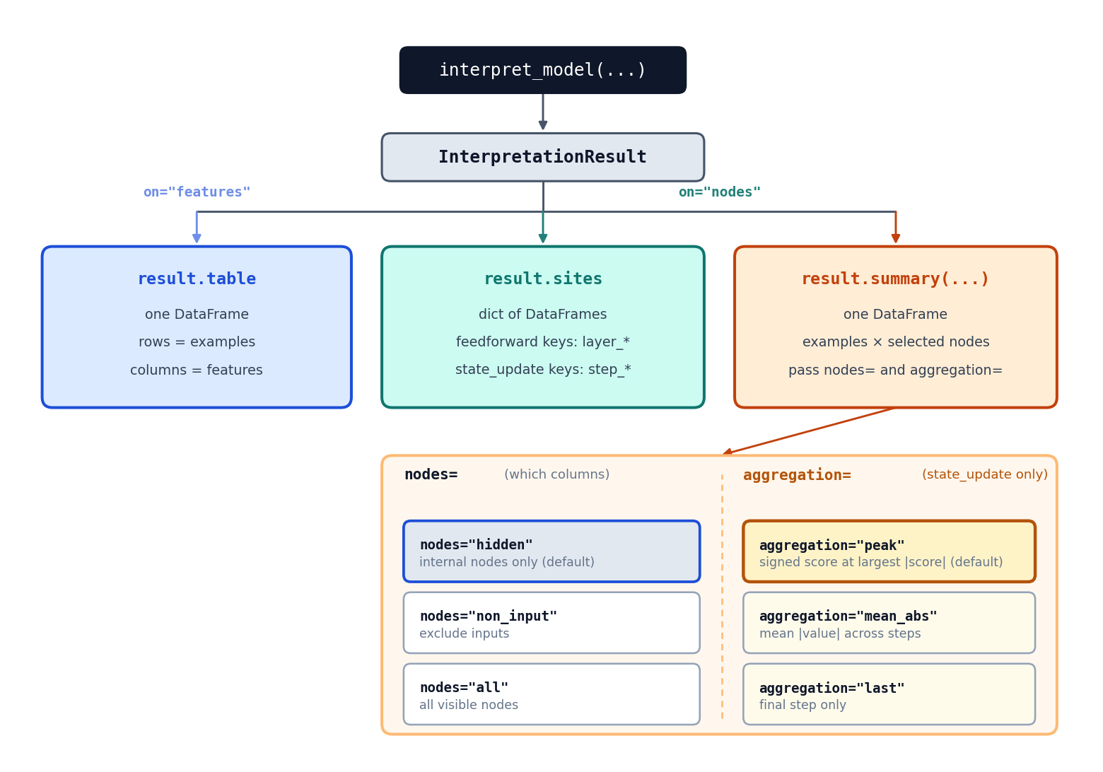
Figure 1. Views on the InterpretationResult returned by
interpret_model(). Feature attribution is one examples-by-features table.
Node attribution is either the raw per-site dictionary or a summary table
whose columns are selected by nodes= and, on state_update, whose repeated
step columns are collapsed by aggregation=. result.table and
result.sites store signed Captum scores. Nothing is abs'd at compute
time; call .abs() yourself if a ranking or plot should use magnitude.
A tiny graph
Two input features feed two hidden nodes, which feed one output. Two examples are enough to see that rows are always examples.
import pandas as pd
import torch
from graphviz import Digraph
from IPython.display import display

import edge2torch as e2t

torch.manual_seed(0)

edgelist = pd.DataFrame(
    {
        "source": ["feat_a", "feat_b", "feat_a", "feat_b", "h1", "h2"],
        "target": ["h1", "h1", "h2", "h2", "y", "y"],
    }
)
data = pd.DataFrame(
    [[0.2, 1.5], [1.1, 0.3]],
    index=["example_0", "example_1"],
    columns=["feat_a", "feat_b"],
)

dot = Digraph()
dot.attr(rankdir="LR")
with dot.subgraph() as subgraph:
    subgraph.attr(rank="same")
    subgraph.node("feat_a")
    subgraph.node("feat_b")
with dot.subgraph() as subgraph:
    subgraph.attr(rank="same")
    subgraph.node("h1")
    subgraph.node("h2")
dot.node("y")
for source, target in edgelist.itertuples(index=False):
    dot.edge(source, target)
dot

A small helper formats every attribution table the same way: caption the shape, label the axes, and color cells so the matrix is readable at a glance. The numbers themselves are untrained toy attributions.
def show_matrix(frame, *, name, rows, columns):
    values = frame.to_numpy(dtype=float)
    vmax = float(abs(values).max()) if values.size else 1.0
    caption = (
        f"{name}  ·  shape {frame.shape[0]} × {frame.shape[1]}"
        f"  ·  rows = {rows}  ·  columns = {columns}"
    )
    styled = (
        frame.style.format("{:.3f}")
        .background_gradient(cmap="RdBu_r", axis=None, vmin=-vmax, vmax=vmax)
        .set_caption(caption)
        .set_properties(
            **{
                "text-align": "center",
                "font-family": "ui-monospace, monospace",
                "font-size": "0.9em",
            }
        )
    )
    display(styled)


model, artifact = e2t.compile_graph(edgelist, backend="feedforward")
print("backend:", artifact.backend)
print("input nodes:", artifact.input_nodes)
print("hidden nodes:", artifact.hidden_nodes)
print("output nodes:", artifact.output_nodes)
print("interpretation sites:", artifact.interpretation_sites)
backend: feedforward
input nodes: ['feat_a', 'feat_b']
hidden nodes: ['h1', 'h2']
output nodes: ['y']
interpretation sites: {'layer_1': ['h1', 'h2'], 'layer_2': ['y']}
On feedforward, interpretation sites start after the input layer. Here that
means layer_1 holds the hidden nodes {h1, h2} and layer_2 holds the
output {y}. Input features are not a node-interpretation site; they appear
in result.table instead.
Feature attributions: result.table
Call interpret_model(..., on="features"). The result's only table is
result.table: one column per input feature, one row per example.
features = e2t.interpret_model(
    model=model,
    artifact=artifact,
    data=data,
    on="features",
    method="IntegratedGradients",
)

print("result.on:", features.on)
print("type(result.table):", type(features.table).__name__)
show_matrix(
    features.table,
    name="result.table",
    rows="examples",
    columns="features",
)
result.on: features
type(result.table): DataFrame
| feat_a | feat_b | |
|---|---|---|
| example_0 | -0.065 | -0.446 |
| example_1 | -0.359 | -0.089 |
Each entry is the attribution of that example's prediction to that input
feature. There is no site axis and no summary() call. Accessing
features.sites or features.summary() raises, because those accessors exist
only when on="nodes".
Node attributions: result.sites
Call interpret_model(..., on="nodes"). result.sites is a dictionary
of DataFrames, one per interpretation site. Every table still has examples
as rows. Columns are the visible nodes at that site.
On feedforward, keys are layer_* and the column sets are disjoint: each
node appears in exactly one site, the layer where it is computed.
nodes = e2t.interpret_model(
    model=model,
    artifact=artifact,
    data=data,
    on="nodes",
    method="LayerConductance",
)

print("result.on:", nodes.on)
print("result.sites keys:", list(nodes.sites.keys()))
print()
for site_id, site_table in nodes.sites.items():
    print(
        f"{site_id}: shape {site_table.shape}, "
        f"columns {list(site_table.columns)}"
    )
    show_matrix(
        site_table,
        name=f'result.sites["{site_id}"]',
        rows="examples",
        columns="nodes at this layer",
    )
result.on: nodes
result.sites keys: ['layer_1', 'layer_2']

layer_1: shape (2, 2), columns ['h1', 'h2']
| h1 | h2 | |
|---|---|---|
| example_0 | -0.008 | -0.502 |
| example_1 | -0.002 | -0.446 |
layer_2: shape (2, 1), columns ['y']
| y | |
|---|---|
| example_0 | -0.510 |
| example_1 | -0.447 |
Read this as:
result.sites = {
    "layer_1": DataFrame  (2 examples × 2 nodes: h1, h2),
    "layer_2": DataFrame  (2 examples × 1 node:  y),
}
result.sites always includes every visible node that the compiler exposes
at a site. There is no nodes= or aggregation= argument on .sites.
Collapsing sites: result.summary()
summary() builds one examples-by-nodes DataFrame from result.sites.
On feedforward it concatenates the site tables along columns, so each
node still appears once. aggregation= is ignored.
nodes= selects which of those columns to keep.
hidden = nodes.summary()
non_input = nodes.summary(nodes="non_input")
all_nodes = nodes.summary(nodes="all")

show_matrix(
    hidden,
    name='result.summary()  ·  nodes="hidden" (default)',
    rows="examples",
    columns="hidden nodes",
)
show_matrix(
    non_input,
    name='result.summary(nodes="non_input")',
    rows="examples",
    columns="non-input nodes",
)
show_matrix(
    all_nodes,
    name='result.summary(nodes="all")',
    rows="examples",
    columns="visible nodes present in sites",
)

print("hidden columns:   ", list(hidden.columns))
print("non_input columns:", list(non_input.columns))
print("all columns:      ", list(all_nodes.columns))
| h1 | h2 | |
|---|---|---|
| example_0 | -0.008 | -0.502 |
| example_1 | -0.002 | -0.446 |
| h1 | h2 | y | |
|---|---|---|---|
| example_0 | -0.008 | -0.502 | -0.510 |
| example_1 | -0.002 | -0.446 | -0.447 |
| h1 | h2 | y | |
|---|---|---|---|
| example_0 | -0.008 | -0.502 | -0.510 |
| example_1 | -0.002 | -0.446 | -0.447 |
hidden columns:    ['h1', 'h2']
non_input columns: ['h1', 'h2', 'y']
all columns:       ['h1', 'h2', 'y']
On this feedforward graph, nodes="all" matches nodes="non_input".
Input features never appear as columns in result.sites, so the summary
cannot include them. Feature attributions stay in result.table.
What the filters mean in general:
nodes= |
Columns kept |
|---|---|
"hidden" (default) |
Internal graph nodes only (h1, h2) |
"non_input" |
Everything except inputs (h1, h2, y) |
"all" |
Every visible node that a site table actually contains |
The same graph on state_update
Compile the same edgelist with steps=2. Node sites are now step_*, and
every step has the same columns: all visible graph nodes, including
inputs. The extra axis is time (update steps), not layer.
su_model, su_artifact = e2t.compile_graph(
    edgelist,
    backend="state_update",
    steps=2,
)
su_nodes = e2t.interpret_model(
    model=su_model,
    artifact=su_artifact,
    data=data,
    on="nodes",
    method="LayerConductance",
)

print("backend:", su_artifact.backend)
print("result.sites keys:", list(su_nodes.sites.keys()))
for site_id, site_table in su_nodes.sites.items():
    show_matrix(
        site_table,
        name=f'result.sites["{site_id}"]',
        rows="examples",
        columns="all visible nodes",
    )
backend: state_update
result.sites keys: ['step_1', 'step_2']
| feat_a | feat_b | h1 | h2 | y | |
|---|---|---|---|---|---|
| example_0 | 0.000 | 0.000 | 0.079 | -0.016 | 0.000 |
| example_1 | 0.000 | 0.000 | -0.064 | 0.019 | 0.000 |
| feat_a | feat_b | h1 | h2 | y | |
|---|---|---|---|---|---|
| example_0 | 0.000 | 0.000 | 0.000 | 0.000 | 0.063 |
| example_1 | 0.000 | 0.000 | 0.000 | 0.000 | -0.045 |
summary() now aggregates across steps instead of concatenating. Each
node remains one column. aggregation= chooses how the two step values
are reduced. Scores stay signed unless you choose "mean_abs".
hidden_cols = ["h1", "h2"]
step_1 = su_nodes.sites["step_1"].loc[:, hidden_cols]
step_2 = su_nodes.sites["step_2"].loc[:, hidden_cols]

show_matrix(
    step_1,
    name='sites["step_1"] hidden columns',
    rows="examples",
    columns="hidden nodes",
)
show_matrix(
    step_2,
    name='sites["step_2"] hidden columns',
    rows="examples",
    columns="hidden nodes",
)
show_matrix(
    su_nodes.summary(aggregation="peak"),
    name='summary(aggregation="peak")  (default)',
    rows="examples",
    columns="hidden nodes",
)
show_matrix(
    su_nodes.summary(aggregation="mean_abs"),
    name='summary(aggregation="mean_abs")',
    rows="examples",
    columns="hidden nodes",
)
show_matrix(
    su_nodes.summary(aggregation="last"),
    name='summary(aggregation="last")  ·  equals step_2',
    rows="examples",
    columns="hidden nodes",
)
| h1 | h2 | |
|---|---|---|
| example_0 | 0.079 | -0.016 |
| example_1 | -0.064 | 0.019 |
| h1 | h2 | |
|---|---|---|
| example_0 | 0.000 | 0.000 |
| example_1 | 0.000 | 0.000 |
| h1 | h2 | |
|---|---|---|
| example_0 | 0.079 | -0.016 |
| example_1 | -0.064 | 0.019 |
| h1 | h2 | |
|---|---|---|
| example_0 | 0.040 | 0.008 |
| example_1 | 0.032 | 0.009 |
| h1 | h2 | |
|---|---|---|
| example_0 | 0.000 | 0.000 |
| example_1 | 0.000 | 0.000 |
aggregation= |
What it does to the step axis |
|---|---|
"peak" (default) |
Keep the signed score from the step with largest magnitude |
"mean_abs" |
Average absolute values across steps (drops the sign) |
"last" |
Use the final step only (signed) |
nodes= still filters columns. On state-update, nodes="all" does
include input features, because they are columns of every step_* table.
Notebooks that plot .abs() do that only for ranking; the stored tables
are signed.
show_matrix(
    su_nodes.summary(nodes="all"),
    name='summary(nodes="all") on state_update',
    rows="examples",
    columns="all visible nodes",
)
print("feedforward summary(nodes='all') columns:", list(all_nodes.columns))
print(
    "state_update summary(nodes='all') columns:",
    list(su_nodes.summary(nodes="all").columns),
)
| feat_a | feat_b | h1 | h2 | y | |
|---|---|---|---|---|---|
| example_0 | 0.000 | 0.000 | 0.079 | -0.016 | 0.063 |
| example_1 | 0.000 | 0.000 | -0.064 | 0.019 | -0.045 |
feedforward summary(nodes='all') columns: ['h1', 'h2', 'y']
state_update summary(nodes='all') columns: ['feat_a', 'feat_b', 'h1', 'h2', 'y']
Choosing a view
| You want | Call | Shape |
|---|---|---|
| Attribution onto input features | interpret_model(..., on="features") then result.table |
examples × features |
| Raw per-layer or per-step node tables | on="nodes" then result.sites |
dict of (examples × nodes at that site) |
| One node table | result.summary(nodes=..., aggregation=...) |
examples × selected nodes |
result.sites is the full visible-node record. result.summary() is the
convenience collapse. aggregation= only changes state-update summaries;
feedforward summaries concatenate disjoint layer columns. Scores in
result.table and result.sites are signed.