Getting started
What does edge2torch do?
edge2torch builds sparsely connected PyTorch neural networks from prior-knowledge graphs,
with optional feature- and node-level attribution.
The core idea is to describe a model structure as a graph: each row in an
edgelist defines a directed connection from a source node to a target node.
edge2torch compiles this graph into a sparsely-connected PyTorch model that
can be trained with ordinary PyTorch tools.
Here, "graph" means the architecture specification, not necessarily a graph neural network. Feedforward models and topology-preserving state-update models can both be represented by edge lists when their architecture is defined through directed connections between named nodes.
This is useful whenever a sparsely-connected neural architecture is known before training and can be represented as named edges.
Domain example: knowledge-primed neural networks
One important use case is a knowledge-primed neural network (KPNN). In a KPNN, prior knowledge encoded as a graph constrains the structure of a neural network. Instead of starting from a fully generic architecture, the model structure is informed by known relationships between named entities.
This is useful because the hidden nodes of the neural network can be designed to correspond directly to meaningful domain entities. In a biological KPNN, for example, hidden nodes may represent transcription factors, kinases, pathways, or other biological processes. After training, attribution methods can then assign importance scores not only to input features, but also to these hidden nodes. Because the hidden nodes are mapped one-to-one to named biological entities, node-level attributions can be interpreted as attributions for those entities . This approach makes the neural networks interpretable.
The figure below illustrates this idea in a biological setting, where entities such as genes, transcription factors, kinases, pathways, and phenotypes can be connected through prior knowledge.
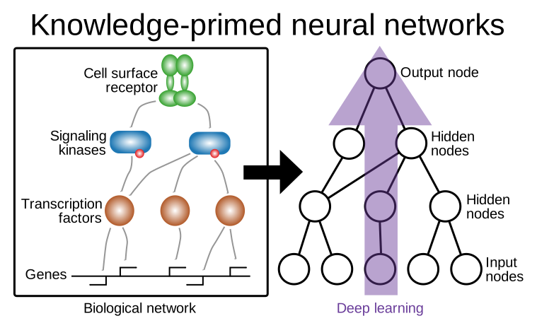
Figure 1. In a pathway-based KPNN, prior biological knowledge is encoded directly into the neural network topology. Hidden nodes represent named biological entities such as receptors, kinases, transcription factors, or pathways, input nodes for example are genes, and edges represent curated regulatory or signaling interactions. This creates a sparsely-connected neural network in which information flow is constrained by the provided biological graph, and attribution scores for neural network nodes can be mapped back to the corresponding biological entities.
Examples of such biologically informed neural networks include pathway-based models as in Fortelny and Bock, 2020 and ontology-based models such as in Elmarakeby et al., 2021.
This is one domain-specific example of the broader edge2torch abstraction:
if a model architecture can be written as named edges, it can potentially be
compiled into a PyTorch model and interpreted back in the space of its named
features and nodes.
The edge2torch workflow
The figure below summarizes the overall edge2torch workflow.

Starting point is a graph that describes the neural network architecture. In
edge2torch, this graph is represented as an edge list, where each row defines
a directed connection between named nodes. compile_graph() turns this edge
list into a minimally opinionated PyTorch model.
The compiled model can then be used like any other PyTorch nn.Module. You can
customize it with customize_model() or with ordinary PyTorch code by adding
activation functions, dropout, task-specific heads, or other downstream modules.
Training is also handled with standard PyTorch tools: losses, optimizers, and
training loops remain under user control.
After training, interpret_model() can compute feature-level or node-level
attributions. It uses the selected Captum attribution method and maps the
results back to the named features and nodes from the original edge list.
This notebook shows a basic edge2torch workflow:
- represent a model architecture as an edgelist
- compile the graph into a PyTorch model
- use the compiled model like ordinary PyTorch
- interpret the trained model back in the space of named features and nodes
The example uses biological names because KPNNs are a natural application area, but the same workflow applies to other domains where the architecture can be expressed as a graph.
Imports
import numpy as np
import pandas as pd
import seaborn as sns
import torch
from graphviz import Digraph
from IPython.display import display
from torch import nn

import edge2torch as e2t
sns.set_theme(style="whitegrid")
Step 1: define a prior-knowledge graph
Currently, edge2torch expects an edgelist with two required columns,
source and target.
Here we define a small feedforward biological graph with two clearly separated branches:
- a signal branch, connected to informative input features
- a noise branch, connected to uninformative input features
This makes the later interpretation steps easier to understand: after training, informative features and their connected hidden nodes should receive stronger attributions than the uninformative branch.
edgelist = pd.DataFrame(
    {
        "source": [
            "gene_signal_1",
            "gene_signal_2",
            "gene_signal_3",
            "gene_noise_1",
            "gene_noise_2",
            "gene_noise_3",
            "tf_signal",
            "tf_noise",
            "kinase_signal",
            "kinase_noise",
        ],
        "target": [
            "tf_signal",
            "tf_signal",
            "tf_signal",
            "tf_noise",
            "tf_noise",
            "tf_noise",
            "kinase_signal",
            "kinase_noise",
            "output_1",
            "output_1",
        ],
    }
)

edgelist
| source | target | |
|---|---|---|
| 0 | gene_signal_1 | tf_signal |
| 1 | gene_signal_2 | tf_signal |
| 2 | gene_signal_3 | tf_signal |
| 3 | gene_noise_1 | tf_noise |
| 4 | gene_noise_2 | tf_noise |
| 5 | gene_noise_3 | tf_noise |
| 6 | tf_signal | kinase_signal |
| 7 | tf_noise | kinase_noise |
| 8 | kinase_signal | output_1 |
| 9 | kinase_noise | output_1 |
# Visualize the graph

dot = Digraph()
dot.attr(rankdir="LR")

input_nodes = [
    "gene_signal_1",
    "gene_signal_2",
    "gene_signal_3",
    "gene_noise_1",
    "gene_noise_2",
    "gene_noise_3",
]
layer_1_nodes = ["tf_signal", "tf_noise"]
layer_2_nodes = ["kinase_signal", "kinase_noise"]
output_nodes = ["output_1"]

with dot.subgraph() as s:
    s.attr(rank="same")
    for node in input_nodes:
        s.node(node, node)

with dot.subgraph() as s:
    s.attr(rank="same")
    for node in layer_1_nodes:
        s.node(node, node)

with dot.subgraph() as s:
    s.attr(rank="same")
    for node in layer_2_nodes:
        s.node(node, node)

with dot.subgraph() as s:
    s.attr(rank="same")
    for node in output_nodes:
        s.node(node, node)

for _, row in edgelist.iterrows():
    dot.edge(row["source"], row["target"])

dot

Step 2: compile the graph
compile_graph(...) returns:
- a compiled PyTorch model
- a compilation artifact containing the metadata needed later for interpretation
torch.manual_seed(1)

model, artifact = e2t.compile_graph(
    edgelist=edgelist,
    backend="feedforward",
)

type(model), type(artifact)
(edge2torch.nn.model.EdgeModel, edge2torch.compile.artifact.CompileArtifact)
Inspect the artifact
The artifact is the compilation record returned alongside the PyTorch model. It
stores the backend, input feature order, and named node roles (input_nodes,
hidden_nodes, output_nodes, interpretation_sites). The compiled model's
execution plan is private. Use edge_weights(model) for the effective
forward-pass weight of each original named graph edge.
artifact.backend
'feedforward'
artifact.feature_names
['gene_noise_1',
 'gene_noise_2',
 'gene_noise_3',
 'gene_signal_1',
 'gene_signal_2',
 'gene_signal_3']
artifact.interpretation_sites
{'layer_1': ['tf_noise', 'tf_signal'],
 'layer_2': ['kinase_noise', 'kinase_signal'],
 'layer_3': ['output_1']}
e2t.edge_weights(model)
| source | target | weight | |
|---|---|---|---|
| 0 | gene_signal_1 | tf_signal | -0.049988 |
| 1 | gene_signal_2 | tf_signal | 0.113232 |
| 2 | gene_signal_3 | tf_signal | 0.020140 |
| 3 | gene_noise_1 | tf_noise | 0.210355 |
| 4 | gene_noise_2 | tf_noise | -0.180192 |
| 5 | gene_noise_3 | tf_noise | -0.079144 |
| 6 | tf_signal | kinase_signal | -0.002825 |
| 7 | tf_noise | kinase_noise | -0.051554 |
| 8 | kinase_signal | output_1 | -0.427065 |
| 9 | kinase_noise | output_1 | -0.263331 |
Step 3: simulate data and align it to the compiled model
The compiled model expects input features in the exact order stored in
artifact.feature_names. In practice, input data often comes from a DataFrame or
AnnData object where features are named but not necessarily ordered like the
model input layer.
align_features_to_input_nodes() uses the compilation artifact to reorder named
input features into the tensor layout expected by the model. This prevents
silent feature-order mismatches between the data and the compiled architecture.
For this tutorial, we first simulate a small binary classification dataset. The
gene_signal_* features carry class information, while the gene_noise_*
features are uninformative. We achieve this by sampling every feature from a normal distribution: the gene_signal_* features use a different mean in each class, so there is a real class difference the model can exploit, while the gene_noise_* features use the same mean in both classes, so any apparent difference between the classes is only random sampling variation.
# Simulate the training and test data
rng = np.random.default_rng(1)

informative_features = [
    "gene_signal_1",
    "gene_signal_2",
    "gene_signal_3",
]

noise_features = [
    "gene_noise_1",
    "gene_noise_2",
    "gene_noise_3",
]

all_features = informative_features + noise_features

n_train_per_class = 100
n_test_per_class = 50


def simulate_binary_classification_data(n_per_class, rng):
    x0_signal = rng.normal(
        loc=0.0,
        scale=1.0,
        size=(n_per_class, len(informative_features)),
    )
    x1_signal = rng.normal(
        loc=2.0,
        scale=1.0,
        size=(n_per_class, len(informative_features)),
    )

    x0_noise = rng.normal(
        loc=0.0,
        scale=1.0,
        size=(n_per_class, len(noise_features)),
    )
    x1_noise = rng.normal(
        loc=0.0,
        scale=1.0,
        size=(n_per_class, len(noise_features)),
    )

    x0 = np.concatenate([x0_signal, x0_noise], axis=1)
    x1 = np.concatenate([x1_signal, x1_noise], axis=1)

    x = np.concatenate([x0, x1], axis=0)
    y = np.concatenate(
        [
            np.zeros(n_per_class, dtype=int),
            np.ones(n_per_class, dtype=int),
        ]
    )

    permutation = rng.permutation(len(y))
    x = x[permutation]
    y = y[permutation]

    x_df = pd.DataFrame(x, columns=all_features)
    y_series = pd.Series(y, name="label")

    return x_df, y_series


x_train_df, y_train = simulate_binary_classification_data(
    n_per_class=n_train_per_class,
    rng=rng,
)

x_test_df, y_test = simulate_binary_classification_data(
    n_per_class=n_test_per_class,
    rng=rng,
)

display(x_train_df.head())
display(y_train.head())
display(x_test_df.head())
display(y_test.head())
| gene_signal_1 | gene_signal_2 | gene_signal_3 | gene_noise_1 | gene_noise_2 | gene_noise_3 | |
|---|---|---|---|---|---|---|
| 0 | 0.382930 | -0.875721 | -1.514319 | 0.287017 | -0.578793 | -0.876897 |
| 1 | 1.517455 | 1.217601 | 1.815758 | 0.163509 | 0.816011 | -2.110056 |
| 2 | 0.245773 | -0.746653 | 0.678740 | 0.878297 | 1.253826 | -0.411778 |
| 3 | 1.760951 | 2.510922 | 3.001886 | -0.288594 | -1.136983 | -0.619579 |
| 4 | 0.663658 | 1.972474 | 0.209167 | 0.759971 | 0.203371 | 1.658664 |
0    0
1    1
2    0
3    1
4    0
Name: label, dtype: int64
| gene_signal_1 | gene_signal_2 | gene_signal_3 | gene_noise_1 | gene_noise_2 | gene_noise_3 | |
|---|---|---|---|---|---|---|
| 0 | 0.096989 | -0.170139 | 0.267756 | 0.777494 | -1.892990 | -0.051819 |
| 1 | 0.840300 | 1.595801 | 2.247646 | -0.166935 | -0.075523 | -0.681671 |
| 2 | -0.046298 | 0.553205 | 0.538196 | 1.204293 | -0.605907 | -0.042248 |
| 3 | 1.802631 | 1.617305 | 3.093590 | -1.421344 | 0.028217 | -1.256497 |
| 4 | 0.855323 | -1.541040 | -0.419259 | 2.527698 | 0.303440 | 1.674191 |
0    0
1    1
2    0
3    1
4    0
Name: label, dtype: int64
# Visualize the simulated training data

import matplotlib.pyplot as plt
import seaborn as sns

plot_df = x_train_df.copy()
plot_df["label"] = y_train.values
plot_df["class"] = plot_df["label"].map({0: "class 0", 1: "class 1"})

long_df = plot_df.melt(
    id_vars=["label", "class"],
    value_vars=artifact.feature_names,
    var_name="feature",
    value_name="value",
)

feature_type_map = {
    "gene_signal_1": "informative",
    "gene_signal_2": "informative",
    "gene_signal_3": "informative",
    "gene_noise_1": "uninformative",
    "gene_noise_2": "uninformative",
    "gene_noise_3": "uninformative",
}

long_df["feature_type"] = long_df["feature"].map(feature_type_map)

g = sns.catplot(
    data=long_df,
    x="class",
    y="value",
    col="feature",
    col_wrap=3,
    hue="class",
    kind="box",
    sharey=False,
    height=3.2,
    aspect=1.0,
    legend=False,
)

g.fig.suptitle(
    "Simulated training data: informative vs. uninformative features",
    y=0.98,
)

g.fig.subplots_adjust(top=0.82, hspace=0.35)

for ax, feature in zip(g.axes.flat, artifact.feature_names):
    feature_type = feature_type_map[feature]
    ax.set_title(f"{feature}\n({feature_type})")
    ax.set_xlabel("")
    ax.set_ylabel("value")

plt.show()

x_train = e2t.align_features_to_input_nodes(
    data=x_train_df,
    artifact=artifact,
)

x_test = e2t.align_features_to_input_nodes(
    data=x_test_df,
    artifact=artifact,
)

x_train.shape, x_test.shape
(torch.Size([200, 6]), torch.Size([100, 6]))
To verify that alignment is based on feature names, we deliberately reverse the DataFrame columns and align the shuffled DataFrame again. The result is identical to the original aligned tensor.
# Alignment is name-based, not position-based.
# Even if the DataFrame columns are shuffled, the aligned tensor is unchanged.

shuffled_columns = list(reversed(artifact.feature_names))
x_train_df_shuffled = x_train_df[shuffled_columns]

x_train_from_shuffled = e2t.align_features_to_input_nodes(
    data=x_train_df_shuffled,
    artifact=artifact,
)

torch.allclose(x_train, x_train_from_shuffled)
True
Keep the compiled input order
PyTorch never sees feature names. Column i is whatever name is in
artifact.feature_names[i]. Keep this model with this artifact,
and build every train/val/test tensor with
align_features_to_input_nodes(..., artifact=artifact).
Do not pass df.values (or any hand-built array) into the model:
if the width is right, training still runs and the features are
silently wired to the wrong nodes. Extra columns and shuffled
DataFrame order are fine; renaming required columns is not.
Step 4: customize the compiled model
The compiled model is intentionally minimal. It defines the graph-derived structural core, but it does not impose architectural choices such as activation functions, dropout, or output heads.
For this binary classification example, we add a one-dimensional linear head that outputs a single logit.
We do not add a downstream ReLU here. The compiled graph already ends in a single output node, and applying ReLU to this scalar bottleneck can suppress gradients into the graph if the output is negative. The linear head keeps the example simple while making the model suitable for binary classification with standard PyTorch loss functions.
customized_model = e2t.customize_model(
    model=model,
    head=nn.Linear(1, 1),
)

customized_model
CustomizedEdgeModel(
  (base_model): EdgeModel(
    (blocks): ModuleList(
      (0-2): 3 x FeedforwardLayerBlock(
        (linear): ConstrainedMaskedLinear()
      )
    )
  )
  (head): Linear(in_features=1, out_features=1, bias=True)
)
Step 5: train the compiled and customized model in PyTorch
The customized model is still a normal PyTorch module. This means it can be trained with ordinary PyTorch components such as loss functions, optimizers, and training loops.
Below is a minimal training step that shows how the compiled structural core and the added architectural components fit directly into a standard PyTorch workflow.
# Train the model with the simulated data

x_train = torch.tensor(
    x_train_df[artifact.feature_names].values,
    dtype=torch.float32,
)
y_train_tensor = torch.tensor(
    y_train.values.reshape(-1, 1),
    dtype=torch.float32,
)

optimizer = torch.optim.Adam(
    customized_model.parameters(),
    lr=1e-2,
)
loss_fn = nn.BCEWithLogitsLoss()

n_epochs = 150
loss_history = []

customized_model.train()

for epoch in range(n_epochs):
    optimizer.zero_grad()

    logits = customized_model(x_train)
    loss = loss_fn(logits, y_train_tensor)

    loss.backward()
    optimizer.step()

    loss_history.append(loss.item())

print("Loss before first update:", round(loss_history[0], 4))
print("Loss after final update: ", round(loss_history[-1], 4))

plt.figure(figsize=(6, 4))
plt.plot(range(1, n_epochs + 1), loss_history)
plt.xlabel("Epoch")
plt.ylabel("Binary cross-entropy loss")
plt.title("Training loss")
plt.tight_layout()
plt.show()
Loss before first update: 0.6963
Loss after final update:  0.0577

Step 6: feature-level interpretation
Feature-level interpretation maps attributions back to the input features.
For this example, we use on="features" and
method="IntegratedGradients".
interpret_model() returns an InterpretationResult. For features, use
result.table (rows are examples, columns are features). Those values
are signed Captum scores. The mean_abs_attribution column below is
computed with .abs() for ranking; it is not how the API stores the
result.
Because the dataset was simulated, we know which features truly separate the
two classes: the gene_signal_* features were generated with different class
means, whereas the gene_noise_* features were not.
This gives us a useful sanity check for interpretation. The recovered feature attributions do not need to match the simulated class mean differences exactly, but the informative features should generally receive larger attribution magnitudes than the uninformative ones.
feature_attr = e2t.interpret_model(
    model=customized_model,
    artifact=artifact,
    data=x_test_df,
    on="features",
    method="IntegratedGradients",
).table

feature_attr.head()
| gene_noise_1 | gene_noise_2 | gene_noise_3 | gene_signal_1 | gene_signal_2 | gene_signal_3 | |
|---|---|---|---|---|---|---|
| 0 | -0.149702 | -0.228903 | 0.018503 | 0.198181 | -0.417863 | 0.663634 |
| 1 | 0.032142 | -0.009132 | 0.243402 | 1.717015 | 3.919306 | 5.570787 |
| 2 | -0.231880 | -0.073267 | 0.015085 | -0.094603 | 1.358677 | 1.333919 |
| 3 | 0.273672 | 0.003412 | 0.448653 | 3.683382 | 3.972121 | 7.667459 |
| 4 | -0.486694 | 0.036692 | -0.597798 | 1.747713 | -3.784814 | -1.039132 |
# Summarize feature attributions and compare them to the simulated signal

class_mean_diff = (
    x_test_df.loc[y_test == 1].mean() - x_test_df.loc[y_test == 0].mean()
)

feature_summary = pd.DataFrame(
    {
        "feature": artifact.feature_names,
        "abs_class_mean_difference": (
            class_mean_diff.abs().reindex(artifact.feature_names).values
        ),
        "mean_abs_attribution": (
            feature_attr.abs()
            .mean(axis=0)
            .reindex(artifact.feature_names)
            .values
        ),
        "mean_signed_attribution": (
            feature_attr.mean(axis=0).reindex(artifact.feature_names).values
        ),
    }
)

feature_type_map = {
    "gene_signal_1": "informative",
    "gene_signal_2": "informative",
    "gene_signal_3": "informative",
    "gene_noise_1": "uninformative",
    "gene_noise_2": "uninformative",
    "gene_noise_3": "uninformative",
}

feature_summary["feature_type"] = feature_summary["feature"].map(
    feature_type_map
)

feature_summary
| feature | abs_class_mean_difference | mean_abs_attribution | mean_signed_attribution | feature_type | |
|---|---|---|---|---|---|
| 0 | gene_noise_1 | 0.094806 | 0.155169 | -0.019322 | uninformative |
| 1 | gene_noise_2 | 0.319823 | 0.102062 | 0.003031 | uninformative |
| 2 | gene_noise_3 | 0.204747 | 0.283213 | -0.019432 | uninformative |
| 3 | gene_signal_1 | 2.111796 | 2.958739 | 1.838984 | informative |
| 4 | gene_signal_2 | 2.164730 | 3.633557 | 2.449118 | informative |
| 5 | gene_signal_3 | 2.159934 | 3.772523 | 2.598134 | informative |
# Plot recovered attributions against the true simulated signal

plot_df = feature_summary.melt(
    id_vars=["feature", "feature_type"],
    value_vars=[
        "abs_class_mean_difference",
        "mean_abs_attribution",
    ],
    var_name="metric",
    value_name="value",
)

plt.figure(figsize=(10, 5))
sns.barplot(
    data=plot_df,
    x="feature",
    y="value",
    hue="metric",
)
plt.xticks(rotation=45, ha="right")
plt.xlabel("feature")
plt.ylabel("magnitude")
plt.title("Feature attributions recover the informative features")
plt.tight_layout()
plt.show()

Step 7: node-level interpretation
Node-level interpretation maps attribution scores back to the internal nodes of the compiled graph.
For this example, we use on="nodes" and method="LayerConductance".
For nodes, result.summary() returns one table with hidden nodes only by
default. Rows are test examples and columns are named graph nodes.
Those values are signed. The plots below use .abs() so we can compare
overall importance when signs would otherwise cancel.
This is often the most interesting interpretation level, because it helps show which hidden biological entities in the network carry signal for the task.
Because this dataset was simulated with informative and uninformative feature groups, we expect nodes on the informative branch of the graph to tend to show larger attribution magnitudes than nodes on branches driven mainly by noise.
node_result = e2t.interpret_model(
    model=customized_model,
    artifact=artifact,
    data=x_test_df,
    on="nodes",
    method="LayerConductance",
)
node_importance = node_result.summary()

node_importance.head()
| tf_noise | tf_signal | kinase_noise | kinase_signal | |
|---|---|---|---|---|
| 0 | -0.359709 | 0.443468 | -0.359709 | 0.443468 |
| 1 | 0.266122 | 11.194892 | 0.266122 | 11.194893 |
| 2 | -0.289745 | 2.595162 | -0.289745 | 2.595161 |
| 3 | 0.724946 | 15.306261 | 0.724946 | 15.306259 |
| 4 | -1.046658 | -3.072880 | -1.046658 | -3.072880 |
Per-site node attribution tables are available with result.sites. For
feedforward models, site keys are layer names such as "layer_1". Those
tables include the visible graph nodes at that site. Feedforward sites start
after the input layer, so input features are not included; use result.table
for inputs.
node_attr_by_site = node_result.sites

for layer_name, layer_df in node_attr_by_site.items():
    print(layer_name)
    display(layer_df.head())
layer_1
| tf_noise | tf_signal | |
|---|---|---|
| 0 | -0.359709 | 0.443468 |
| 1 | 0.266122 | 11.194892 |
| 2 | -0.289745 | 2.595162 |
| 3 | 0.724946 | 15.306261 |
| 4 | -1.046658 | -3.072880 |
layer_2
| kinase_noise | kinase_signal | |
|---|---|---|
| 0 | -0.359709 | 0.443468 |
| 1 | 0.266122 | 11.194893 |
| 2 | -0.289745 | 2.595161 |
| 3 | 0.724946 | 15.306259 |
| 4 | -1.046658 | -3.072880 |
layer_3
| output_1 | |
|---|---|
| 0 | 0.083759 |
| 1 | 11.461016 |
| 2 | 2.305416 |
| 3 | 16.031206 |
| 4 | -4.119538 |
To make the node-level results easier to interpret, we now summarize the attributions across the test set.
For each node, we compute:
- the mean attribution
- the mean absolute attribution
The mean absolute attribution is often especially useful, because it reflects
overall importance even when positive and negative values cancel out on average.
That .abs() step is a display choice; result.sites and result.summary()
keep the signed scores.
node_summary_frames = []

for layer_name, layer_df in node_attr_by_site.items():
    layer_summary = pd.DataFrame(
        {
            "layer": layer_name,
            "node": layer_df.columns,
            "mean_attribution": layer_df.mean(axis=0).values,
            "mean_abs_attribution": layer_df.abs().mean(axis=0).values,
        }
    )
    node_summary_frames.append(layer_summary)

node_summary = (
    pd.concat(node_summary_frames, ignore_index=True)
    .sort_values(
        ["layer", "mean_abs_attribution"],
        ascending=[True, False],
    )
    .reset_index(drop=True)
)

node_summary
| layer | node | mean_attribution | mean_abs_attribution | |
|---|---|---|---|---|
| 0 | layer_1 | tf_signal | 6.878730 | 9.126179 |
| 1 | layer_1 | tf_noise | -0.035684 | 0.320601 |
| 2 | layer_2 | kinase_signal | 6.878730 | 9.126178 |
| 3 | layer_2 | kinase_noise | -0.035684 | 0.320601 |
| 4 | layer_3 | output_1 | 6.843048 | 9.144727 |
The following plot shows the mean absolute attribution for each internal node across the test set. Magnitude is used here only so the ranking is easy to read.
plot_df = node_summary.sort_values(
    "mean_abs_attribution",
    ascending=True,
)

plt.figure(figsize=(9, 5))
sns.barplot(
    data=plot_df,
    x="mean_abs_attribution",
    y="node",
    hue="layer",
    dodge=False,
)
plt.xlabel("Mean absolute node attribution")
plt.ylabel("Node")
plt.title("Node-level attribution summary on the test set")
plt.tight_layout()
plt.show()

Control: swap which branch is informative
The main example already pairs a positive and negative control in one experiment: the signal branch lights up and the noise branch stays low. The architecture is symmetric, so that contrast is fairly strong on its own.
One remaining check is a swap control: put class signal on the former
noise genes instead. If attribution tracks the data rather than branch
identity, importance should move to tf_noise / kinase_noise, while the
former signal branch should drop.
This section is intentionally short: same graph, swapped informative features, retrain, and compare node importance.
# Control: class signal on the former noise genes.
torch.manual_seed(11)
rng_swap = np.random.default_rng(11)

swap_informative = [
    "gene_noise_1",
    "gene_noise_2",
    "gene_noise_3",
]
swap_uninformative = [
    "gene_signal_1",
    "gene_signal_2",
    "gene_signal_3",
]
swap_features = swap_informative + swap_uninformative


def simulate_swap(n_per_class, rng):
    n_inf = len(swap_informative)
    n_noise = len(swap_uninformative)
    x0 = np.concatenate(
        [
            rng.normal(0.0, 1.0, size=(n_per_class, n_inf)),
            rng.normal(0.0, 1.0, size=(n_per_class, n_noise)),
        ],
        axis=1,
    )
    x1 = np.concatenate(
        [
            rng.normal(2.0, 1.0, size=(n_per_class, n_inf)),
            rng.normal(0.0, 1.0, size=(n_per_class, n_noise)),
        ],
        axis=1,
    )
    x = np.concatenate([x0, x1], axis=0)
    y = np.concatenate(
        [
            np.zeros(n_per_class, dtype=int),
            np.ones(n_per_class, dtype=int),
        ]
    )
    perm = rng.permutation(len(y))
    return (
        pd.DataFrame(x[perm], columns=swap_features),
        pd.Series(y[perm], name="label"),
    )


x_swap_train_df, y_swap_train = simulate_swap(100, rng_swap)
x_swap_test_df, y_swap_test = simulate_swap(50, rng_swap)

swap_model, swap_artifact = e2t.compile_graph(
    edgelist=edgelist,
    backend="feedforward",
)
swap_model = e2t.customize_model(
    model=swap_model,
    head=nn.Linear(1, 1),
)

x_swap_train = e2t.align_features_to_input_nodes(
    data=x_swap_train_df,
    artifact=swap_artifact,
)
y_swap_tensor = torch.tensor(
    y_swap_train.values.reshape(-1, 1),
    dtype=torch.float32,
)

optimizer = torch.optim.Adam(swap_model.parameters(), lr=1e-2)
loss_fn = nn.BCEWithLogitsLoss()
swap_model.train()
for _ in range(150):
    optimizer.zero_grad()
    loss = loss_fn(swap_model(x_swap_train), y_swap_tensor)
    loss.backward()
    optimizer.step()

swap_node_attr = e2t.interpret_model(
    model=swap_model,
    artifact=swap_artifact,
    data=x_swap_test_df,
    on="nodes",
    method="LayerConductance",
).summary()

swap_summary = (
    swap_node_attr.abs()
    .mean(axis=0)
    .rename("mean_abs_attribution")
    .reset_index()
    .rename(columns={"index": "node"})
)
branch_map = {
    "tf_signal": "signal branch",
    "kinase_signal": "signal branch",
    "tf_noise": "noise branch",
    "kinase_noise": "noise branch",
    "output_1": "output",
}
swap_summary["branch"] = swap_summary["node"].map(branch_map)

# Compare against the main-example node summary when available.
main_internal = (
    node_summary.loc[
        node_summary["node"].isin(branch_map),
        ["node", "mean_abs_attribution"],
    ]
    .groupby("node", as_index=False)["mean_abs_attribution"]
    .max()
    .rename(columns={"mean_abs_attribution": "main_example"})
)
compare = main_internal.merge(
    swap_summary[["node", "mean_abs_attribution", "branch"]],
    on="node",
    how="outer",
).rename(columns={"mean_abs_attribution": "swap_control"})
compare = compare.sort_values("swap_control", ascending=False)
display(compare)

plt.figure(figsize=(7, 3.5))
sns.barplot(
    data=swap_summary.sort_values(
        "mean_abs_attribution",
        ascending=True,
    ),
    x="mean_abs_attribution",
    y="node",
    hue="branch",
    dodge=False,
)
plt.xlabel("Mean absolute node attribution")
plt.ylabel("Node")
plt.title("Swap control: signal on former noise branch")
plt.tight_layout()
plt.show()
| node | main_example | swap_control | branch | |
|---|---|---|---|---|
| 0 | kinase_noise | 0.320601 | 7.743877 | noise branch |
| 3 | tf_noise | 0.320601 | 7.743877 | noise branch |
| 1 | kinase_signal | 9.126178 | 0.782549 | signal branch |
| 4 | tf_signal | 9.126179 | 0.782549 | signal branch |
| 2 | output_1 | 9.144727 | NaN | NaN |

If the swap worked, mean absolute attribution should concentrate on the
noise-branch nodes (tf_noise, kinase_noise) rather than the
signal-branch nodes (tf_signal, kinase_signal). That confirms the quiet
noise branch in the main example reflected uninformative inputs, not a
structural preference for the left-hand pathway.